Practical 4 - Local Illumination
Objectives of this practical:
introduce lighting in your scenes
improve your understanding of illumination models
implement the Phong illumination model, as seen in the lecture
Pre-requisites:
it is best but not mandatory to have completed Practical 2 - Meshes and modeling
you can have a look at the GLSL tips page to get familiar with additional GLSL operations needed for this practical (
normalize(),dot(),reflect(),pow()…)
For this practical, we provide a new set of files
viewer.py
phong.vert
phong.frag,
to be used with the
core.py
transform.py
given in the previous practicals.
The provided viewer.py is a very simple skeleton
to load objects from files using the generic load() function,
provided in the core.py utilities and render them all with the Phong
shader. We now work with complete implementations of Mesh and
Viewer from core.py.
For this practical, you will thus be mainly working on the GLSL shader code.
Most 3D file formats are able to
specify Phong parameters, for example .obj files have sister material files
with .mtl extension which store these parameters in readable ASCII format.
For testing, you can find different material samples in
this material file.
To use, insert the following lines with any material name found in the above
file, at the head of the
suzanne.obj 3D file:
mtllib vp.mtl
usemtl aqua
Exercices
1. The Lambertian model
Until now, we mostly studied how to create complex geometry and how to use OpenGL functions to manipulate shaders and buffers on the GPU. Today, you will mainly work on the shaders themselves using the GLSL programming language.
Your first task will be to implement the Lambertian model, defined at any surface point by the following function:
\(I = K_d (\mathbf{n} \cdot \mathbf{l})\),
where \(K_d\) is the color of the object (also called albedo or diffuse color), \(\mathbf{l}\) is the direction of the light (a unit vector) and \(\mathbf{n}\) is the normal of the surface.
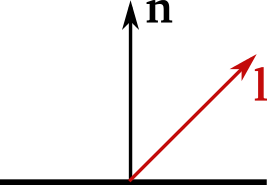
This function will have to be written in the fragment shader to obtain the final rendering. The light vector defined is passed as a uniform variable. Make also sure to take the following remarks into account to obtain a proper result:
as shown in the figure above, the convention is to use only vectors directed outward with respect to the object surface.
if the light is located under the surface, the scalar product will result a negative value and should thus be clamped to 0.
after being rasterized, the normal might not be a unit vector anymore. Make sure to re-normalize it in the fragment shader.
the illumination computation must be done with data located in the same coordinate frame. If the normal is defined in the camera frame, the light direction must be expressed in the same space.
Note
Passing the NIT matrix
In case of non-uniform scaling, the model and view matrices cannot be used
directly to transform normal vectors. As seen in lecture 1,
the proper way to tranform a normal is to use the NIT matrix:
\((M^{-1})^\top\) where \(M\) is the upper left 3x3 matrix of
the modelview matrix. Look up the inverse() and transpose()
GLSL functions to do it in GPU, or use numpy.linalg.inv() and
a.T to transpose a Numpy array a on the CPU side.
2. The Phong model
The Phong model uses an additional term that accounts for specular reflections:
\(I = K_a + K_d (\mathbf{n} \cdot \mathbf{l}) + K_s (\mathbf{r} \cdot \mathbf{v})^s\),
where \(K_a\) is a constant ambient color that approximates complex inter-reflections between objects in the scene by a constant term, and \(K_s\) is the color of highlights, or specular color (usually white). The exponent \(s \in (0,\infty)\) is the shininess and controls the shape of the specular lobe. Tiny lobes (or mirror-like) surfaces are obtained with high values of \(s\).
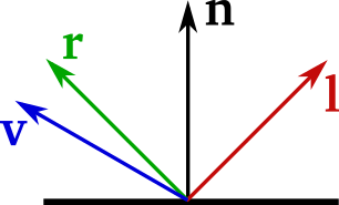
\(\mathbf{r}\) is the reflected light vector and can easily be computed
using the GLSL built-in reflect() function. The view vector
\(\mathbf{v}\) can be either given as a uniform variable or directly
computed in the shader via the model and view matrices. Note that a position
defined in camera space (after the transformation by the model and view
matrices) already provides a non-normalized view vector. Once again, be careful
with negative values that must be clamped to 0 (a shading function should not
create negative energy).
Optional Exercises
The exercises below are all independent except 4 and 5.
3. Control light and shading parameters
Level: easy
Assign some key handlers to control the parameters of the Phong model. You may want to change the color of the surface (\(K_d\)) or to modify the shininess \(s\) for instance.
Animate the light direction \(\mathbf{l}\) in such a way that it rotates
around the scene. Hint: a uniform timer will be necessary in the shader to
compute the new direction at each frame, which you can retrieve with
glfw.get_time().
4. Point light
Level: medium
Previous exercices only consider a directional light (where the direction is the same everywhere on the surface). This definition is usually used when considering distant lights, such as the sun.
The goal here is to use a point light instead, for which the direction changes locally. Moreover, its intensity decreases with the square of the distance between the surface and the light. Formally, the Phong model becomes:
\(I = K_a + \frac{1}{d^2} [K_d (\mathbf{n} \cdot \mathbf{l}) + K_s (\mathbf{r} \cdot \mathbf{v})^s]\),
where \(d\) is the distance between the position of the light and the surface point at which the illumination is computed.
5. Multiple lights
Level: easy
Complex scenes usually use multiple lights to obtain more realistic renderings. Your goal is to define and animate/control 2 or more directional and/or point lights. The equation becomes:
\(I = K_a + \sum_k \frac{1}{d_k^2} [K_d (\mathbf{n} \cdot \mathbf{l_k}) + K_s (\mathbf{r_k} \cdot \mathbf{v})^s]\).
When using multiple lights, the result is simply computed as the sum of all contributions. You may try to assign a different color to each light in order to see them separatly in the rendering.
Elements of solution
We provide a discussion about the exercises in Practical 4 - Elements of solution. Check your results against them.